
This post is one in a long series of posts that I will be making on Reinforcement Learning. The posts will largely follow a book that I am reading, namely “Reinforcement Learning, An Introduction“, by Richard S. Sutton, and Andrew G. Barto, second edition, The MIT Press. There is a great Reinforcement Learning Specialization from coursera that goes along with (did you know that you can audit any coursera course and get access to everything but the graded assignments and the certificate?). If you have the taste for a more rigorous presentation, then there is this NPTEL course from my alma mater (did you know that you can actually register for courses on NPTEL website, get certificates from IITs, and use the credits in several universities, all for Rs. 1000 per course, i.e. for < $14 !!).
The k-armed Bandit Problem
The k-armed bandit problem, or the multi-armed bandit problem is the Hello-world of RL. In the k-armed bandit problem, there are k arms or actions that you can choose from, and each action provides a reward that is sampled from an unknown distribution. In the least complicated setting, the distribution is unknown, but stationary. The entity making these action choices is called the “agent”. The goal of the agent is to choose actions so as to maximize the expected reward.
This problem would be trivial if the distribution of rewards corresponding to each action was known. In that case one could choose the distribution with the largest expected reward. Similarly, the problem would be trivial if we were only interested in the expected reward after a long time horizon. In that case the agent could try each action a large number times and estimate the expected reward values to desired accuracy. Thereafter, they could select the action with largest expected reward. The issue is that the reward distributions unknown, and we do care about the transient behavior.
Below we discuss the most common approaches to resolving the explore-exploit dilemma. The notation used here is described on this page.
Explore-Exploit Algorithms
1. Epsilon-Greedy Exploration
Under an epsilon-greedy exploration policy, the agent chooses the action which has the highest estimated reward with probability 1-ε, and chooses one of the remaining actions with probability ε. Thus, the agent explores all actions, while also exploiting the action with the best estimated reward. Note that this policy will never converge to an optimal policy. Also note that larger values of ε mean more exploration, and smaller asymptotic reward.
2. Optimistic Initial Values
Under this approach we set the initial estimate of all the rewards to some large optimistic value, and use a greedy policy from thereon. As actions are explored, and value estimates revised, it is guaranteed that the agent will explore all actions. This policy is guaranteed to converge to optimal reward given sufficient time.
3. Upper-Confidence-Bound Selection

Under this scheme, the action taken at timestep ‘t’ is decided according to the above formula. Here, Q_t(a) is the current estimate of the reward from action ‘a’, N_t(a) is the number of times the action ‘a’ has been explored in the past, and ‘c’ is a constant. Thus, Upper-Confidence-Bound, or UCB, ensures that each action is taken at least once, and has reasonable performance in practice.
Reward Updates
For all the algorithms described above, the agent takes an action ‘a’, receives a reward ‘r’, and then has to update their knowledge about the world based on the action-reward pair. Suppose the agent summarizes their knowledge of the world in form of the expected reward from each action. Then they can use the following update procedure.
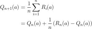
We assume here that the sum only runs for those time indices ‘i’ where the action ‘a’ was sampled. The equation above is of a general form that will be used repeatedly in RL,
NewEstimate = OldEstimate + StepSize * (Target – OldEstimate)
Conclusion
Thats it for bandits! Using these ideas you can almost up to date with the state of art of bandit problems. Implement your own bandits and have fun!
